Training a large neural network is influenced by a great many factors. Switching the optimizer, changing the model architecture, or using a different training set can all lead to drastically different results.

In engineering practice, we jokingly refer to the empirical process of tuning these factors as "alchemy."

But how can we move from experience to laws, and describe the relationships among these factors more accurately and quantitatively? If we can figure this out, our alchemy will be much more grounded.

"Scaling Law" attempts to answer this question in a relatively quantitative way.

Since OpenAI's foundational work in 2020 (Kaplan Law[1]), Scaling Law has become one of the most reliable empirical laws in deep learning. It can be used to estimate model performance, guide hyperparameter selection, and judge the effectiveness of a given change. To this end, many works have also attempted to provide deeper, more essential interpretations of Scaling Law.

This article also shares the author's understanding of Scaling Law.

Preparation

In the following sections, we will repeatedly encounter problems of the form "find the minimum of a power-law combination under a given constraint," so in this section we first prepare two basic conclusions.

The Cross-Power Inequality

First, we introduce the most frequently used inequality. Let , then

The condition for equality is

This can be proven using the simple inequality [2].

Below we demonstrate the latter. The weighted AM-GM inequality is , so we have

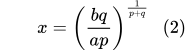
The condition for equality is , i.e., 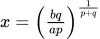. For convenience, we call this inequality the "cross-power inequality." Its main feature is that it involves two power functions whose exponents have opposite signs.

More interestingly, both the minimum point and the minimum value themselves remain power laws, which is one of the cornerstones for the subsequent derivations.

The Optimal Allocation Ratio

The cross-power inequality fixes the product () and finds the minimum of the sum of two power-law terms. There are also scenarios (such as finding the optimal allocation ratio for parameter counts) where we need to fix their "sum" to find the minimum. Specifically, let ; we want to solve

Unfortunately, this problem has no elementary closed-form solution, but numerical solving is straightforward. It is not hard to see that a minimum must exist. Substituting and taking the derivative gives . Setting it to zero yields

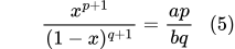
The left-hand side is clearly monotonically increasing with respect to on the interval . When , the left-hand side tends to ; when , it tends to 0. By the intermediate value theorem, there exists a unique solution in , which can be obtained directly by bisection.

Conceptual Framework

The training process of a model can be formalized as

> Given data , architecture , and optimizer , minimize the loss function .

Here, denotes some ideal distribution, which can also be imagined as an extremely large test set. Any training set we can construct is a subset of it, or equivalently, a sampled result. represents the loss value that the model can achieve on the ideal distribution under these conditions.

Triple Decomposition

We consider the following decomposition:

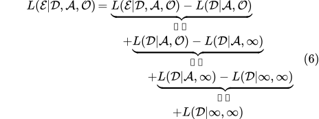
At first glance, this decomposition seems to complicate the problem, but in fact it breaks down the distance from the current training state to the ideal target into three progressively nested steps.

Under the conventional assumption that "more is better," each bracket is non-negative. Therefore, this is equivalent to writing the total gap as a sum of three individually interpretable distances, which decouples the influence of each variable on the loss function as much as possible, allowing us to more reasonably infer the dependencies among them.

Now let us explain the meaning of each term in the formula one by one.

Data Error

The first-level decomposition is

where represents the loss value of the model on the training set given the architecture and optimizer .

Note that by definition, represents the loss of the model on the ideal distribution , which is our ultimate goal.

However, is untouchable during training. We can only interact with the training set , so we can only obtain the training loss , and then try to describe the gap between them via .

This term is also commonly called the "generalization error." Its key influencing factor is the data—such as the quantity, quality, and diversity of the data. In addition, the architecture and optimizer may also change the generalization error. Which variables to consider specifically depends on our analysis goals.

Optimization Error

The second-level decomposition is

where represents the ideal loss achievable on the training set when optimization is pushed to the extreme—for example, with a perfect super-optimizer, or by pushing the number of training steps and tuning iterations to infinity.

Thus, represents the ceiling of the optimizer, while measures the distance between the practical optimizer and this ceiling. It assesses whether the optimizer is good enough—for example, whether the learning rate is appropriate, whether the number of training steps is sufficient, whether the batch size stabilizes the gradient, and so on.

Architecture Error

The third-level decomposition is

where represents the most ideal loss achievable on the training set when both optimization and architecture are pushed to the extreme—with any excellent optimizer and any powerful model.

Thus, is the theoretical limit determined by the current data itself, while measures the gap between the practical model and its theoretical limit. It assesses whether the architecture is good enough—whether the parameter count is sufficient, whether the depth and width are adequate, whether there is still room for improvement in residual connections, and so on.

Optimization

In this section, we first explore the optimization gap .

Given an optimizer (such as Adam or Muon), we mainly care about the influence of three core parameters: the learning rate , the batch size , and the number of training steps .

Of course, in theory, other parameters such as momentum and other details could also be considered, but here we mainly focus on these three parameters.

Relationship Analysis

First, a reasonable assumption is that "the more you train, the better the result." Here, "training more" includes both "more steps" and "larger learning rate." Alternatively, we can intuitively think that is the "distance traveled" by the model. The longer the distance traveled, the better the result, so we can guess that there is a contribution of the form .

On the other hand, training performance is also affected by noise, and a reasonable assumption is that the larger the noise, the worse the performance. Noise comes from two sources: one is the batch size , where a smaller batch size means more noise; the other is the learning rate, which represents the degree of nonsmoothness of the training process—the larger it is, the more noise it implies. So we conjecture that there is another term .

Adding these two parts together gives

We can also understand the above equation by dividing the training process into two stages: in the early stage, noise is secondary, and the term allows the loss function to drop quickly first; afterward, noise gradually takes effect, and the model begins to oscillate near the target point, resembling a spiral descent trajectory.

This form is consistent with those used in 2503.12645[3] and 2603.15958[4]. It is worth pointing out that these two works are not based on experimental fitting, but rather on direct theoretical analysis of the convergence of optimizers such as SignSGD and Muon, with the conclusion being . In the subsequent derivation, we can substitute these numerical values for a simple verification.

Optimal Learning Rate

Equation (10) contains 6 parameters. If we directly fit it, we would need to sample a very large number of points, which would be extremely costly and also highly prone to overfitting. To address this, we can leverage the optimal-parameter assumption to further simplify the form.

First, using the power-mean inequality, we can find the optimal learning rate that minimizes the right-hand side:

The corresponding minimum value is

This tells us two results: 1. There exists some such that the optimal learning rate is inversely proportional to ; 2. Assuming we can always find the optimal learning rate for each configuration, the asymptotic law of the optimization error can be simplified to the form , reducing the number of parameters to 4. This is precisely the decoupled form proposed in 2607.01487[5], while 2605.09154[6], derived from a noisy quadratic model, also concludes that should be modeled separately.

Optimal Batch Size

Now, starting from the optimal-learning-rate assumption, we set the optimization error to

Let , which denotes the number of samples seen during training. Note that we do not restrict Multi-Epoch, so it is possible that some samples are learned multiple times. If we fix , then the right-hand side becomes . Again, using the power-mean inequality, we can obtain the minimum value:

This also yields two conclusions: given a fixed total number of training samples , the optimal batch size is proportional to , where ; and under the optimal batch size, the Scaling Law simplifies to , which is exactly the classical Scaling Law form.

Summary

We can now summarize: the general Scaling Law for optimizers is . If we assume training is always run at the optimal learning rate, it simplifies to . If we further fix the number of training samples and assume the optimal batch size can always be found, it simplifies to .

As for the optimal parameters, the optimal batch size is proportional to a power no greater than 1 of , which is consistent with the Step Law; the optimal learning rate is inversely proportional to a power no greater than 1 of . Converting according to , the optimal learning rate is also inversely proportional to a power no greater than 1 of , which is consistent with the Microsoft Law but opposite to the Step Law.

If we substitute the theoretical values mentioned earlier, , then we have , and consequently , which is still fairly close to the given by the Step Law.

In addition, we have ). Converting according to gives , which is also not far from the of the Microsoft Law.

Finally, there is ), which is also very close to the given by the Chinchilla Law.

Architecture Section

Next, we turn to the model gap ), which purely discusses the contribution of the architecture to the loss function. Classic variables include the parameter count , width , depth , and so on. At the same time, the introduction of architecture variables in turn affects the variation pattern of the optimization gap, and we will try to sort out all these aspects as much as possible.

Model Parameters

Given a fixed overall architecture, the main variable of the model is the parameter count . Assuming that a larger parameter count leads to better performance, it is reasonable to posit

This is the most basic assumption of the Scaling Law with respect to parameter count, consistent with the Kaplan Law and the Chinchilla Law. Among them, the Kaplan Law gives , while the Chinchilla Law gives a fitted result of . It is currently widely believed that the Chinchilla Law is more accurate as the training scale grows.

A point of contention here is whether the parameter count ) should include the Embedding. The mainstream practice is to exclude it, but this may lead to significant deviations at small scales, which could be one of the reasons for the discrepancy between the Kaplan Law and the Chinchilla Law (in the era of Kaplan's experiments, training scales were generally small). Paper 2406.12907[7] provides a detailed analysis of this issue. For a more accurate treatment of the contribution of Embedding, refer to the later section "Memory Layer."

Besides compressing the entire architecture into a single parameter count , we can be more fine-grained. For example, we can separate width and depth to study whether a "tall and thin" or "short and wide" model is better:

Since the model parameter count is roughly , we can, under a fixed parameter count, find the optimal width, height, and the corresponding :

Paper 2606.25008[8], based on theoretical work (2505.10465[9], 2602.05970[10]), proposes . Substituting this in gives

The final is still very close to the Chinchilla Law.

Optimization Laws

Meanwhile, changes in parameter count also affect the optimization process. In Eq. (10), the three coefficients are treated as constants, which assumes a given architecture . Now that we introduce the parameter count , then naturally becomes a function of as well.

We again understand this in two parts:

On one hand, the larger the parameter count, the stronger the model's capacity, and the faster the loss function decreases, so we replace with ;

On the other hand, the larger the parameter count, the more complex the model, and the greater the noise it introduces, so we replace with and , respectively, giving

Here a natural question arises: why do we only consider how varies with , but not how the exponents vary? We will defer this question to the "Power Law" section. Now, repeating the calculations from the "Optimization" section, we obtain

If we accept results such as Kaplan Law[1], Chinchilla Law[11], and Step Law[12], then and are independent of . By setting the exponents of these two terms to zero, we can solve

Substituting into the various expressions, we find that only one new parameter is introduced:

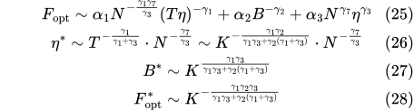
Interestingly, the form of is exactly consistent with Microsoft Law[13], meaning it is negatively correlated with both and . This is not trivial, because we only assumed that and are independent of , with no assumption about . Finally, substituting the theoretical values , we obtain

As for , Microsoft Law gives , while Step Law gives . Given that these two Laws have completely opposite dependencies on , it is normal that they differ significantly in this exponent.

The theory leans somewhat more toward Microsoft Law. From some convex optimization results, is related to the standard deviation of the gradients of all parameters, so we speculate it lies between . Combined with Microsoft Law, we can estimate a value of .

Given Compute Budget

Combining and , we have

For dense models, the computation per step is essentially proportional to the parameter count . Here, is the number of samples seen during training, which is also proportional to the training compute, so the total computational cost consumed during training is . The proportionality constant for a standard architecture is roughly , including for the forward pass and for the backward pass.

In practice, compute is usually limited. We want to maximize intelligence under a fixed compute budget , which means we need to find the optimal and under the constraint . Substituting into the above equation (absorbing constant factors into the coefficients), we obtain

This again takes the form of a heterogeneous power inequality, so we directly apply the formula to get

If we substitute the earlier theoretical values and , then

This is very close to the core conclusion of Chinchilla Law: the optimal model size and the optimal amount of data should scale roughly proportionally (the paper's fitted result is ).

Finally, substituting the expressions for and into the and from the previous section, we obtain

Here, is not too far from the in DeepSeek Law[14], but DeepSeek Law gives , whereas even substituting here only yields , which is still somewhat far off.

From this perspective, the various results are fairly consistent on the optimal batch size, but they diverge significantly on the optimal learning rate, which may be closely related to specific optimization settings and learning rate schedules.

Sparse Architectures

Earlier we said that "compute is roughly proportional to the parameter count ," which holds for dense models. Assuming the core operation of the model is a Linear layer, where the input of is multiplied by the parameters of , the compute is and the parameter count is . Both are proportional to , so the parameter count equals the compute. However, in recent years, there has been growing interest in architectures that decouple parameter count from compute, such as MoE.

MoE is undoubtedly the dominant architecture today—almost every open-source large model is an MoE. One important new parameter it introduces is sparsity , which can be defined as the ratio of total parameters to activated parameters, or the ratio of total experts to activated experts.

From a theoretical standpoint, the theoretical compute of MoE depends roughly only on the number of activated parameters. In other words, increasing sparsity does not increase compute in theory, while loss can still decrease, so increasing sparsity is always worthwhile.

A simple way to incorporate sparsity into the Scaling Law is:

where are the activated parameter count and total parameter count, respectively, and . A similar form also appears in 2501.12370[15].

If we look at Equation (16), this is equivalent to assuming that only affects the coefficient in a power-law manner, but does not affect the exponent . From the above equation, we can also derive the concept of "effective parameter count":

That is, an MoE model with activated parameter count and total parameter count is equivalent to a Dense model with parameter count .

This concept originates from the Effective Parameter Count proposed in 2202.01169[16]. Later, Ling Law[17] further extended it into an "efficiency lever" and explored how it varies.

However, since compute is only proportional to the activated parameter count , this means we could keep unchanged while letting . In other words, we could reduce compute to nearly zero while keeping performance unchanged, but this seems unrealistic.

Therefore, a reasonable guess is that should include an additional penalty term involving to ensure a certain level of activated parameters:

Other works that model sparsity include 2309.08520[18], 2501.12370[15], and 2502.05172[19], each of which sets a different form of Scaling Law.

Beyond sparsity, the granularity of Experts (first modeled in 2402.07871[20]) and Shared Experts also have some impact on performance. Work 2509.23678[21] combines all these factors into a very large form for experimental fitting.

Of course, "increasing sparsity is always worthwhile" is only true in theory. In practice, routing overhead, inference efficiency, and other issues must also be considered. Increasing sparsity is not entirely free and requires co-design between algorithms and infrastructure.

The Layer of Memory

Besides MoE, another way to decouple parameter count from compute is through sparse Memory layers. Classic examples include PKM[22] and UltraMem[23], while newer approaches such as Over-Encoding[24] and Engram also fall into this category.

In fact, these works can be viewed as another extreme of MoE: their "Experts" are simplified to trainable vectors with no computation, and a trainable Router (Pointer) or N-gram Hash is used to select which "Experts" to activate.

From this perspective, their Scaling Law should be similar to that of MoE. For example, when a Dense model is augmented with several Memory layers, the Scaling Law should still take the form of Equation (37).

If these two different types of sparse designs—MoE and Memory—are used simultaneously, what should the Scaling Law look like? Let us first define a few notations , representing "activated parameter count (counting only parameters that incur compute, i.e., the Dense part plus activated Experts)", "total parameter count after removing Memory", "total parameter count after removing inactive Experts", and "total parameter count", respectively. They satisfy the identity

If we guess that the effects of MoE and Memory are complementary, then their Scaling Law might be additive, i.e.,

This also leads to a new optimization problem: if we must fix the activated parameter count (compute bottleneck) and the total parameter count (memory bottleneck), how should we allocate parameters between MoE and Memory?

According to the identity (38), is then a constant, and we need to minimize the above under this constraint.

Let . Substituting this into the above equation, the problem becomes the constrained minimization problem introduced in the "Optimal Allocation Ratio" section, which can be solved numerically.

That is, it is not optimal to allocate all parameters to either MoE or Memory; rather, there exists an optimal ratio, which is similar to the finding in Engram[25].

A Brief Summary

Similar to the optimization section, this section first makes power-law assumptions based on empirical observations, and then mainly uses the heterogeneous power inequality for optimization calculations.

The simplest variable for quantifying a model is the total parameter count . For finer granularity, we can consider width and depth separately.

Under the Dense model assumption, the parameter count itself also represents compute, and the optimizer's training steps and batch size are also positively correlated with compute. We can then explore how to determine the optimal parameter count and corresponding optimizer settings under a fixed total budget .

If we refine further, there are even more architectural variables. For example, MoE architectures distinguish between "activated parameters" and "total parameters," and Memory designs such as Engram are similar. When both appear together, there is also the problem of optimal parameter allocation. We have not yet mentioned residual improvements such as MHC[26] and AttnRes[27], among others. In short, the variables that can be considered on the model side are very numerous, and we can only briefly touch on them here.

Data Section

Finally, we turn to the data gap . By definition, this term requires us to focus on performance under the ideal distribution , but we have also said that the ideal distribution is theoretically unreachable. So how do we measure it?

In fact, there is no particularly good method. We can only choose a test set that has not been trained on and that we believe is sufficiently representative, and use the test loss computed on it as an approximation of . Therefore, similar to benchmarks, the construction of the test set is especially important, as it represents how well we understand and describe the ideal target.

Data size #The core hyperparameter for data is the size of the training set . We believe that a larger training set leads to better generalization performance (i.e., "the more you see, the more you know"), so it contributes a term .

Each step's data is uniformly randomly sampled from the training set, so is the average number of times each sample is trained on, i.e., the number of training epochs. We believe that the more severe the Multi-Epoch, the worse the generalization performance, so it contributes a term . Thus, a basic form is

Most Scaling Law works treat and as the same under the Single-Epoch assumption. This article distinguishes them in order to account for the effects of Multi-Epoch.

A recent paper, Prescriptive Scaling Laws for Data Constrained Training [28], also introduces a similar power law, but replaces with , while also accounting for the effect of model parameter count. The general view is that the larger the model, the more prone it is to overfitting, and therefore the less it should be trained with Multi-Epoch. This leads to a positive correlation between and . These modifications can also be adjusted as needed.

On the other hand, works such as Scaling Data-Constrained Language Models [29] introduce the concept of "value decay," converting the data volume after Multi-Epoch into an "effective data volume" to correct the Scaling Law. However, I feel that this correction is only necessary because those works do not distinguish between and . Since we already distinguish between and , we only need to directly penalize the overfitting risk introduced by Multi-Epoch.

Optimal number of epochs — Combining the optimization error and the data error (fixing and , and assuming training is always performed under optimal hyperparameters), the result is:

This clearly shows: the more training, the smaller the optimization error, but the more severe the data repetition and the larger the generalization error. Therefore, again using the heterogeneous power inequality, we can find the optimal value of :

This provides a scaling law for Multi-Epoch, with the conclusion: the less data available, the more epochs one should train; the more data, the smaller the optimal number of epochs. This conclusion is exactly the opposite of that in 2511.13421 [30].

One possible improvement is to generalize to , in which case we have:

With this formulation, the optimal number of epochs can either increase or decrease as data grows.

However, even with , there are still some unreasonable aspects. For example, when , it also tends to infinity, but empirically, even if we keep training indefinitely, the test loss should not become infinite.

That said, if we only fit within a small range (assuming the number of Multi-Epochs cannot be too large), the power-law assumption may still yield practically usable results.

Further Thoughts

Beyond the core parameter of data volume , many works make fine-grained distinctions about data composition, such as domain mixing ratios (2403.16952 [31], 2507.09404 [32], 2603.19149 [33], 2605.12715 [34], 2606.08167 [35]), quality levels (2510.03313 [36]), and modality ratios (2607.22043 [37]). These works are diverse and difficult to distill into a unified form, so I will not elaborate on each one.

Compared to optimization and architecture, the Scaling Law on the data side indeed feels more "messy" and "fuzzy."

The reason is not hard to understand: the variables for optimizers () and architectures () are relatively well-defined numbers, whereas on the data side, apart from data volume which can be quantified fairly accurately, dimensions such as domain, quality, and modality lack clear boundaries and cannot be precisely characterized by a single scalar.

Moreover, from the notation , it can be seen that are all conditions of it. That is, changes in optimizer variables and architecture variables will, in principle, also affect the data-side Scaling Law. The interaction among various variables makes it difficult to study the data dependence law cleanly under a "well-controlled" setting.

What is even more troubling is that, upon careful reflection, the very proposition of a "Data Scaling Law" is itself puzzling: to fairly measure performance, we first need to prepare a sufficiently representative test set, then "pretend" not to know what the test set looks like, and try to study the "Scaling Law" on the training data so that the test set performance is as good as possible. No matter how one looks at it, this procedure is rather strange.

Summary

In this section, we briefly introduced the Scaling Law for the data gap, mainly introducing the data volume parameter , considering the positive effect of increasing data volume, as well as the overfitting risk introduced by Multi-Epoch, and combined it with the optimization error to derive the optimal number of epochs. Overall, however, the data-side Scaling Law still has many confusing aspects that require deeper investigation.

Power Law Chapter

So far, we have assumed all scaling laws take the form of sums or products of "power laws," and then used the "heterogeneous power inequality" to derive some optimal choices. Looking back now, there are two questions worth considering:

1. Why do we assume the scaling law takes a power-law form? 2. When we introduce additional conditions, why do we only consider changes in the coefficient of the power law, rather than changes in the exponent?

The Question of Power Laws

Why power laws? Many researchers have attempted to provide more "fundamental" explanations, but I feel that many attempts merely replace one assumption with another without substantive change, such as in Deriving Model Scaling Laws Based on Quantization Assumptions [38].

In my view, the most direct explanation is: when we determine that the dependence on a variable is monotonically decreasing and we only care about asymptotic behavior, the number of functions we can choose from is actually limited — generally just power functions and exponential functions.

Exponential functions decay too quickly — in the language of distributions, they are "short-tailed" — meaning that with a small investment of resources, the returns quickly hit a ceiling, which does not match our "intuition" about the real world. Power functions, on the other hand, are "long-tailed": they decay more slowly and better describe the phenomenon of "continuous investment, continuous improvement."

To put it more philosophically, if the world were dominated by exponential functions, it would be too boring: everything would quickly hit a ceiling, and all kinds of investment would quickly lose meaning. It is precisely because power laws dominate that the story of Scale Up becomes vivid.

Another perspective is that power laws are equivalent to "scale invariance": , the function looks the same at any scale, and the very meaning of the word "Scaling" is precisely a law that holds across scales — and the elementary function that can play this role seems to be only the power law.

From a practical standpoint: a power law is a straight line in log-log coordinates, which makes it easier to fit and visualize. Moreover, the existence of the "heterogeneous power inequality," and the fact that its minimum point and minimum value are still power laws, are all important reasons why it can serve as an "empirical law."

Of course, the power law is not the only answer. In the "Data Chapter," some papers use exponential functions to describe the value decay of Multi-Epoch. It can only be said that the power law is the basic law worth trying first in most cases. If we encounter problems that are particularly difficult to fit, we can consider making adjustments. Alternatively, if the extrapolation interval is not large, what may matter more is the monotonicity of the function, and the differences between different functional forms may not be that significant.

The Question of Coefficients

The second question first appeared in the "Architecture Chapter." We assumed that changes in conditions affect at most the coefficient of the power law — for example, architectural changes only affect the coefficient of the optimization-error power law, and changes in MoE sparsity only affect the power law of the architecture error, while the exponent remains unchanged. What is the reasoning behind this? Is there a more fundamental principle involved?

Next is the physical analogy: in statistical physics, the critical exponents of phase transitions are universal. Different materials within the same universality class share the same set of exponents, and material details only change the non-universal prefactor.

Similarly, the exponent of a Scaling Law can be understood as the "difficulty" of the problem itself — it is determined by the data distribution and the task. The coefficient, on the other hand, represents the "engineering level" of the solution — it changes with improvements in the optimizer and architecture. Essentially, this means doing better on the same problem, so what should change is the coefficient in front of the power law, not the exponent.

Conversely, if a finite engineering improvement could truly change the exponent, then in the asymptotic sense, the relative advantage it brings would grow without bound as the scale increases — a finite investment yielding unbounded relative returns would amount to exponential progress out of nowhere, which is usually unrealistic. Unless the improvement changes the problem itself, but then it is no longer "engineering improvement on the same problem" — it is a different problem altogether.

Of course, this is more of a conjecture based on simplicity and self-consistency on my part. It is an open question, and discussion is welcome.

Summary Chapter

After reading this blog post, some readers may feel that "it says everything, yet says nothing." We have not proven any theorems; we have only written down a triple decomposition, empirically posited a set of power-law assumptions, and then used optimization methods to perform some basic analysis.

In this way, we attempted to identify the commonalities among various Scaling Law results and clarify their interaction mechanisms. Fortunately, this article does yield some heuristic results, but limited by the author's expertise, most of the content can only be introduced at a superficial level—especially the "data section," where the author's understanding remains at a very shallow stage.

Walking through the entire derivation process, I personally feel a flavor reminiscent of "dimensional analysis" in physics: it is not as rigorous as first-principles derivation, but instead first guesses the power-law forms of each term based on intuition and monotonicity, then derives the laws governing the optimal solution, and finally compares against classical results for simplification or correction.

I hope the perspective offered here can provide some help to readers in understanding and applying Scaling Laws.

Reference Links

1. Kaplan Law
2. Weighted AM-GM inequality
3. 2503.12645
4. 2603.15958
5. 2607.01487
6. 2605.09154
7. 2406.12907
8. 2606.25008
9. 2505.10465
10. 2602.05970
11. Chinchilla Law
12. Step Law
13. Microsoft Law
14. DeepSeek Law
15. 2501.12370
16. 2202.01169
17. Ling Law
18. 2309.08520
19. 2502.05172
20. 2402.07871
21. 2509.23678
22. PKM
23. UltraMem
24. Over-Encoding
25. Engram
26. MHC
27. AttnRes
28. Prescriptive Scaling Laws for Data Constrained Training
29. Scaling Data-Constrained Language Models
30. 2511.13421
31. 2403.16952
32. 2507.09404
33. 2603.19149
34. 2605.12715
35. 2606.08167
36. 2510.03313
37. 2607.22043
38. Deriving Scaling Laws for Model Size Based on Quantization Assumptions